Thiago Scarelli

How to simulate random draws from any distribution

Sep. 2020

Simulating synthetic data is an easy way to check whether an estimator will work as intended before you have access to real-world data. Indeed, more experienced researchers have told me on different occasions that this step should be part of any research project. The key advantages are that you know exactly how the variables were generated, and your sample is as large as you need it to be. But how do you actually get random draws from a given distribution?

Short answer: in most cases, your statistical software has a built-in function for that. Here is a quick reference:

[R code example] 1000 random draws from a given distribution

# Uniform distribution
draws_uniform <- runif(n = 1000, min = 0, max = 1)
hist(draws_uniform)

# Normal distribution
draws_normal <- rnorm(n = 1000, mean = 0, sd = 1)
hist(draws_normal)

# Binomial distribution
draws_binomial <- rbinom(n = 1000, size = 100, prob = .1)
hist(draws_binomial)

# Exponential distribution
draws_exponential <- rexp(n = 1000, rate = 1)
hist(draws_exponential)

# Weibull distribution
draws_weibull <- rweibull(n = 1000, shape = 2, scale = 2)
hist(draws_weibull)

# Gamma distribution
draws_gamma <- rgamma(n = 1000, shape = 1, scale = 2)
hist(draws_gamma)

[Stata code example] 1000 random draws from a given distribution

// Set the number of observations
set obs 1000

// Uniform distribution with parameters a = 0 and b = 1
gen uniform = runiform(0, 1)

// Normal distribution with parameters m = 0 and s = 1
gen normal = rnormal(0, 1)

// Binomial distribution with parameters n = 100 and p = 0.1
gen binomial = rbinomial(100, 0.1)

// Exponential distribution with parameters b = 1
gen exponential = rexponential(1)

// Weibull distribution with paramters a = 1 and b = 2
gen weibull = rweibullph(1, 2)

// Gamma distribution with paramters a = 1 and b = 2
gen gamma = rgamma(1, 2)

A more general answer

If you need more flexibility, you can simulate random draws for any arbitrary distribution, provided that you can write down an analytical form for the inverse of its cumulative distribution function (CDF). You just need to take this new function and evaluate it using random draws from the standard uniform.

Example: Draws from an exponential distribution

Suppose you need to simulate draws from an exponential distribution (and ignore for the moment that there is a function for that). This distribution is a nice one because it is fully characterized by a single parameter $\lambda$ (often called the rate parameter), and it is helpful in several applications, particularly those related to the modeling of the duration of something.

For non-negative values of $x$, its CDF is given by:

Hence its inverse could be written as:

If you generate random draws $u_i$ from the standard uniform distribution [0, 1] and use them as input in the above function to recover many $x_i = F^{-1}(u_i; \lambda)$, those $x_i$ will follow an exponential distribution of rate $\lambda$.

[R code example]

# How many draws?
N <- 100000

# A vector of n draws from a uniform distribution
u_i <- runif(n = N, min = 0, max = 1)

# Parameter that defines the distribution of interest
lambda <- 2

# Draws from an exponential distribution using the inverse of its CDF
exp_i <- -log(1 - u_i) / lambda

# A density plot with the simulated values
library(ggplot2)
ggplot(as.data.frame(exp_i)) + geom_density(aes(x = exp_i))

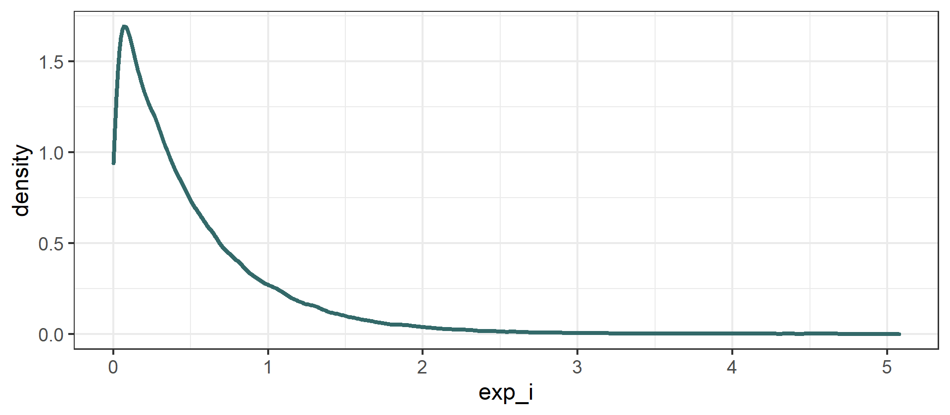
If you check the mean and the standard deviation of exp_i, you should find values close to 0.5 (or, in general, $1/\lambda$). Furthermore, the distribution created this way converges to what you would obtain using R’s function rexp(n = 100000, rate = 2). After all, what the software is doing under the hood is similar to what we are doing explicitly.

[Stata code example]

* How many draws?
set obs 100000

* Draws from a uniform distribution
gen u_i = runiform()

* Parameter that defines the distribution of interest
scalar lambda = 2

* Draws from an exponential distribution using the inverse of its CDF
gen exp_i = -log(1 - u_i) / lambda

* A density plot with the simulated values
kdensity exp_i

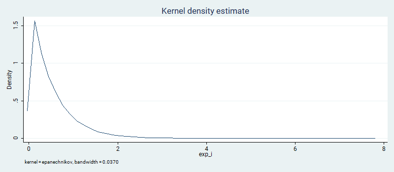
Again, the results are similar to what one would obtain with Stata’s own rexponential(2).

More importantly, the same strategy goes beyond the exponential case and can be generalized for more exotic distributions that do not have a preexisting random function available, or for cases in which the default parametrization is different from the one you would need.

Why does it work?

The CDF, by definition, maps every possible value a function can take into the interval between 0 and 1. Intuitively, the strategy above uses this property: it reverts the mapping from the interval [0, 1] back to the support of the function. The shape of $F^{-1}(\cdot)$ alone is enough to make more frequent values of $x_i$ appear more often, even if every $u_i$ has the same probability of occurring.